(Comments)
In our previous post, we made a model predict if a motor is faulty with its audio recording data. We feed the model with the audio time series data, achieved a decent testing accuracy of 0.9839. In this post, we will discover feeding the model with extracted features from the time series data. The final prediction accuracy improved to 100% with our test WAV file.
The Mel-frequency cepstrum (MFC) is a representation of the short-term power spectrum of a sound, Mel-frequency cepstral coefficients (MFCCs) are coefficients that collectively make up an MFC, MFC wiki.
Enough for the theory, let’s take a look at it visually.
In order to extract MFCC feature from our audio data, we are going to use the Python librosa library.
First, install it with pip
pip install librosa
We are going to use a siren sound WAV file for the demo. Download the siren_mfcc_demo.wav from the Github here and put in your directory
In a Python console/notebook, let’s import what we need first
import librosa
import librosa.display
import matplotlib.pyplot as plt
import numpy as np
plt.style.use('ggplot')
Then let’s extract the MFCC features
def feature_normalize(dataset):
    mu = np.mean(dataset, axis=0)
    sigma = np.std(dataset, axis=0)
    return (dataset - mu) / sigma
siern_wav = "./siren_mfcc_demo.wav"
sound_clip,s = librosa.load(siern_wav)
sound_clip = feature_normalize(sound_clip)
frames = 41
bands = 20
window_size = 512 * (frames - 1)
mfcc = librosa.feature.mfcc(y=sound_clip[:window_size], sr=s, n_mfcc = bands)
feature_normalize function is same as the last post, which normalizes the audio time series to be around 0 and have standard deviation 1.
Let’s visualize the MFCC features, it is a numpy array with shape (bands, frames) i.e. (20, 41) in this case
librosa.display.specshow(mfcc, x_axis='time')
plt.show()
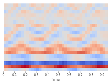
This is the MFCC feature of the first second for the siren WAV file. The X-axis is time, it has been divided into 41 frames, and the Y-axis is the 20 bands. Did you notice any patterns in the graph? We will teach our model to see this pattern as well later.
The model structure will be different from the previous post since the model input changed to
MFCC features.
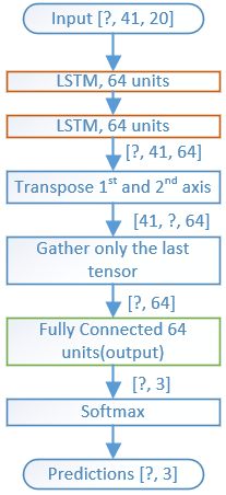
Notice one model input shape matches with one MFCC feature transposed shape (frames, bands) i.e. (41, 20). Mfcc feature is transposed since the RNN model expects time major input.
For the complete source code, check out my updated GitHub. Feel free to leave a comment if you have a question.
Share on Twitter Share on Facebook
Comments