(Comments)

TL;DR
We are building a TensorFlow model to take input of the audio recording on a motor and make a prediction if it is "healthy".
Imagine in a production environment like a warehouse distribution center, there are hundreds of AC motors drives conveyor belts and sorters day and night. Let’s say one motor at a critical joint breaks down, it can cause major downtime of the whole production line. An experienced maintenance engineer can identify a faulty motor by listening to its sounds and take action to correct it before it is too late.
In this demo, we are going to train our model to be an expert. It can tell if a motor is faulty by listening to its sound.
The training data contains 6 WAV files recorded on 3 types of motors in 2 locations.
Recorded in the lab environment with contact piezoelectric disk microphone sandwiched between two magnets. The magnet is then attached to the housing of the AC motor.
You may wonder why we don't just use a normal non-contact microphone?
If you have visited the shop floor of a large distribution center. You might see there are tones of motors/actuators running for many reasons, some are moving the box around, some are putting labels on the box, some are packing/unpacking. Which means it is
Using a contact microphone made with piezoelectric disk make sure the majority of the audio signal recorded is generated by the motor we attached to. Similar to a doctor is placing a stethoscope on your chest.
Here is an image to illustrate the idea.

For the demo purpose, let's simplify the task to just classifying one motor to be one of those three types.
e.g. used_60Hz_re_10s_22khz.wav means,
sound_file_paths = ["new_60Hz_de_10s_22khz.wav","new_60Hz_re_10s_22khz.wav",
                    "used_60Hz_de_10s_22khz.wav","used_60Hz_re_10s_22khz.wav",
                    "red_60Hz_de_10s_22khz.wav","red_60Hz_re_10s_22khz.wav"]
Let's break done the task into the following parts, feel free to jump to sections you are most interested in.
We read the data with module librosa.load() function, which takes one argument- the WAV file path, return a tuple, the first element is a numpy array of audio time series, the second element is the sampling rate.
    sound_clip,sr = librosa.load(sound_file_full_path)
    print("Sampling rate for file \"{}\" is: {}Hz".format(sound_file_path,sr))
Normalize the audio time series to be around 0 and have standard deviation 1. This helps our model to learn much faster later on.
def feature_normalize(dataset):
    mu = np.mean(dataset, axis=0)
    sigma = np.std(dataset, axis=0)
    return (dataset - mu) / sigma
Segment the audio time series.
Our model will be using LSTM recurrent layer which expects fixed-length sequences as input data. Each generated sequence contains 100 timesteps of audio recording.
N_TIME_STEPS = 100 # 22050 sr, --> 4.5ms
N_FEATURES = 1 # one channel audio signal
step = 50
segments = []
labels = []
for i, sound_file_path in enumerate(sound_file_paths):
    label = sound_names[i]
    sound_file_full_path = base_dir+sound_file_path
    sound_clip,sr = librosa.load(sound_file_full_path)
    print("Sampling rate for file \"{}\" is: {}Hz".format(sound_file_path,sr))
    v = feature_normalize(sound_clip)
    for i in range(0, len(v) - N_TIME_STEPS, step):
        segments.append([v[i: i + N_TIME_STEPS]])
        labels.append(label)
The graph illustrates structure of the model.
LSTM layers read the input sequence and finally use fully-connected layer + softmax to make a prediction.
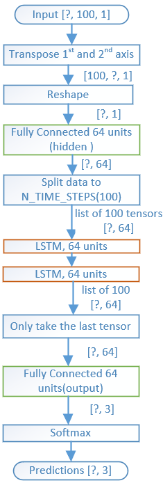
LSTM layer is one type of recurrent network layer which processes the audio time series data.
I find this article below quite useful to develop
Understanding LSTM Networks --
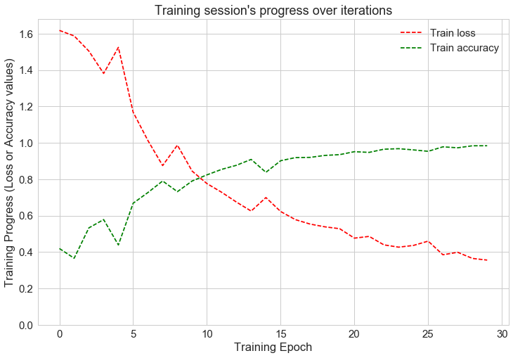
Train for 30 epochs, achieved final training accuracy 0.9843, testing accuracy 0.9839
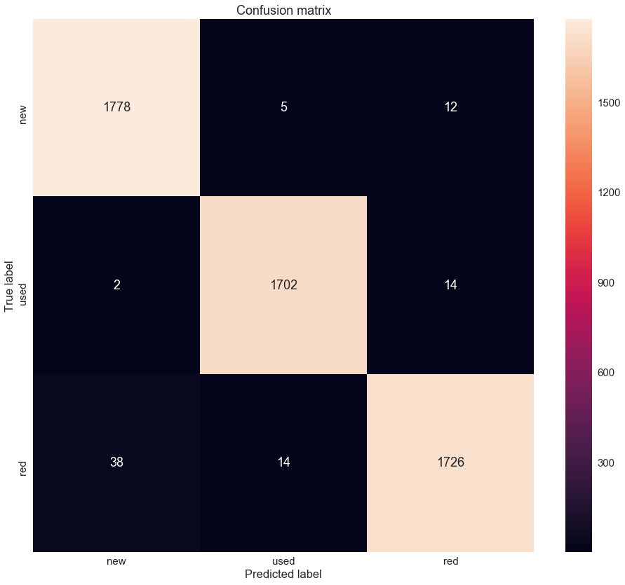
Let's have a look at the confusion matrix for the result. It describes the performance of the trained classifier.
Before we predict our new recordings, we need to save the trained model to file, so next time we just need to simply load it.
Here is the code to "freeze" our trained model to a file
from tensorflow.python.tools import freeze_graph

MODEL_NAME = 'acoustic'

input_graph_path = './model/' + MODEL_NAME+'.pbtxt'
checkpoint_path = './model/' +MODEL_NAME+'.ckpt'
restore_op_name = "save/restore_all"
filename_tensor_name = "save/Const:0"
output_frozen_graph_name = './model/frozen_'+MODEL_NAME+'.pb'

freeze_graph.freeze_graph(input_graph_path, input_saver="",
                          input_binary=False, input_checkpoint=checkpoint_path,
                          output_node_names="y_", restore_op_name=restore_op_name,
                          filename_tensor_name=filename_tensor_name,
                          output_graph=output_frozen_graph_name, clear_devices=True, initializer_nodes="")
And here is the counterpart to load up the "frozen" model so we can use it to do some prediction.
def load_graph(frozen_graph_filename):
    # We load the protobuf file from the disk and parse it to retrieve the
    # unserialized graph_def
    with tf.gfile.GFile(frozen_graph_filename, "rb") as f:
        graph_def = tf.GraphDef()
        graph_def.ParseFromString(f.read())

    # Then, we import the graph_def into a new Graph and returns it
    with tf.Graph().as_default() as graph:
        # The name var will prefix every op/nodes in your graph
        # Since we load everything in a new graph, this is not needed
        tf.import_graph_def(graph_def, name="prefix")
    return graph


graph = load_graph('./model/frozen_acoustic.pb')
After that, we will access the input and output nodes of the loaded graph.
x = graph.get_tensor_by_name('prefix/input:0')
keep_prob = graph.get_tensor_by_name('prefix/keep_prob:0')
y = graph.get_tensor_by_name('prefix/y_:0')
Our new recording will also be a WAV file, so let's have the function to convert it to our model input data.
'''
Segmentment the wav file and return the model input data
'''
def process_wav(filepath):
    N_TIME_STEPS = 100 # 22050 sr, --> 4.5ms
    N_FEATURES = 1 # one channel audio signal
    step = 50
    segments = []
    sound_clip,sr = librosa.load(filepath)
    print("Sampling rate for file \"{}\" is: {}Hz".format(sound_file_path,sr))
    v = feature_normalize(sound_clip)
    for i in range(0, len(v) - N_TIME_STEPS, step):
        segments.append([v[i: i + N_TIME_STEPS]])
    model_input_data = np.asarray(segments, dtype= np.float32).reshape(-1, N_TIME_STEPS, N_FEATURES)
    return model_input_data
Let's also have a helper function so we can call easily to do the prediction
def predict_recording(filepath):
    X_predict = process_wav(filepath)
    # We launch a Session
    with tf.Session(graph=graph) as sess:
        # Note: we don't nee to initialize/restore anything
        # There is no Variables in this graph, only hardcoded constants
        y_predicts = sess.run(y, feed_dict={x: X_predict, keep_prob: 1})
        LABELS = ["new","used","red"]
        predicted_logit = stats.mode(np.argmax(y_predicts,1))[0][0]
        predicted_label = LABELS[predicted_logit]
        predicted_probability = stats.mode(np.argmax(y_predicts,1))[1][0] / len(y_predicts)
        return (predicted_label, predicted_probability)
Whew, that was a lot of code. Let's test it out with our new WAV file, it is another recording from a "new" motor.
predicted, prob = predict_recording(sound_file_full_path)
print("Recording \"{}\" is predicted to be a \"{}\" motor with probability {}".format(sound_file_full_path, predicted, prob))
It correctly predicts this WAV file is a recording of a "new" motor with probability 0.8227,
Sampling rate for file "test_new_60Hz.wav" is: 22050Hz
Recording "./data/test_new_60Hz.wav" is predicted to be a "new" motor with probability 0.8227010881160657
We use Tensorflow to build a model trained on 6 WAV files, recorded on 3 different types of motors. The model can classify new audio recording to the correct motor type.
The dataset is quite small and might only work for this one motor model number running on 60Hz. To overcome this limitation, more data with a variety of motor model numbers can be added to the training dataset as well as different VFD frequency.
Check out my GitHub for source code. Leave a comment if you have any questions or concerns.
Share on Twitter Share on Facebook
Comments