(Comments)
Editor’s Note: Part 1 of this series was published in Hacker Noon. Check it out here
Welcome back to the second part of this series. In this section, we’ll dive into the YOLO object localization model.
Although you’ve probably heard the acronym YOLO before, this one’s different. YOLO stands for "You Only Look Once".
Why "look once" you may wonder? Because there are other object location models that look "more than once," as we will talk about later. The "look once" feature of YOLO, as you already expected, makes the model run super fast.
In this section, we’ll introduce a few concepts: some are unique to the YOLO algorithm and some are shared with other object location models.
The concept of breaking down the images
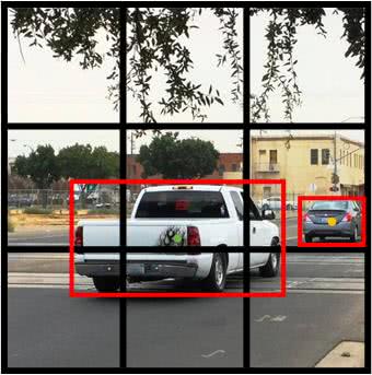
In the image above we have two cars, and we marked their bounding boxes in red.
Next, for each grid cell, we have the following labels for training. Same as we showed earlier in Part 1 of the series.

So how do we associate objects
For the rightmost car, it’s easy. It belongs to the middle right cell since its bounding box is inside that grid cell.
For the truck in the middle of the image, its bounding box intersects with several grid cells. The YOLO algorithm takes the middle point of the bounding box and associates it to the grid cell containing it.
As a result, here are the output labels for each grid cell.
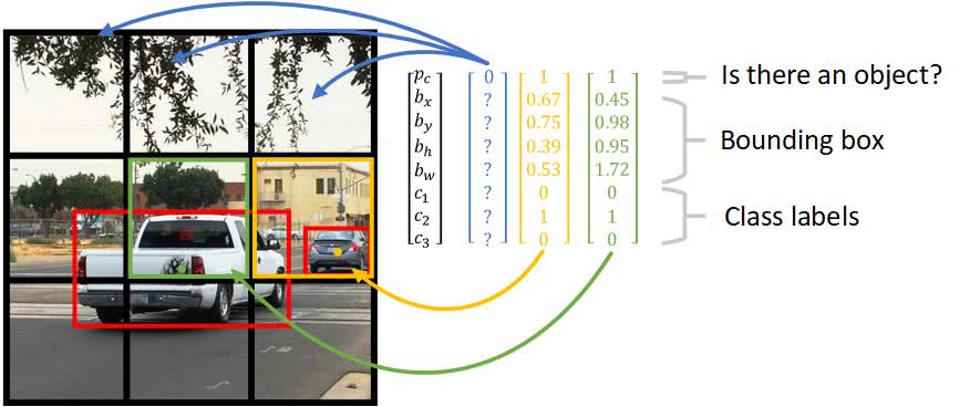
Notice that for those grid cells with no object detected, it’s pc = 0 and we don’t care about the rest of the other values. That’s what the "?" means in the graph.
And the definition of the bounding box parameter is defined as follows:
For the class labels, there are 3 types of targets we’re detecting,
With "car" belonging to the second class, so c2 = 1 and other classes = 0.
In reality, we may be detecting 80 different types of targets. As a result, each grid cell output y will have 5 + 80 = 85 labels instead of 8 as shown here.
With that in mind, the target output combining all grid cells have the size of 3 x 3 x 8.
But there’s a limitation with only having grid cells.
Say we have multiple objects in the same grid cell. For instance, there’s a person standing in front of a car and their bounding box centers are so close. Shall we choose the person or the car?
To solve the problem, we’ll introduce the concept of anchor box.
Anchor box makes it possible for the YOLO algorithm to detect multiple objects centered in one grid cell.
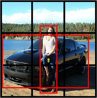
Notice that, in the image above, both the car and the pedestrian are centered in the middle grid cell.
The idea of anchor box adds one more "dimension" to the output labels by pre-defining a number of anchor boxes. So we’ll be able to assign one object to each anchor box. For illustration purposes, we’ll choose two anchor boxes of two shapes.
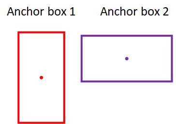
Each grid cell now has two anchor boxes, where each anchor box acts like a container. Meaning now each grid cell can predict up to 2 objects.
But why choose two anchor boxes with two different shapes—does that really matter? The intuition is that when we make a decision as to which object is put in which anchor box, we look at their shapes, noting how similar one object's bounding box shape is to the shape of the anchor box. For the above example, the person will be associated with the tall anchor box since their shape is more similar.
As a result, the output of one grid cell will be extended to contain information for two anchor boxes.
For example, the center grid cell in the image above now has 8 x 2 output labels in total, as shown below.
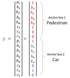
Another reason for choosing a variety of anchor box shapes is to allow the model to specialize better. Some of the output will be trained to detect a wide object like a car, another output trained to detect a tall and skinny object like a pedestrian, and so on.
In order to have a more formal understanding of the intuition of "similar shape", we need to understand how it’s evaluated. That is where the Intersection over Union —comes into play.

The concept of Intersection over Union (
But implementing
Instead of defining a box by its center point, width and height, let's define it using its two corners (upper left and lower right): (x1, y1, x2, y2)
To compute the intersection of two boxes, we start off by finding the intersection area's two corners. Here’s the idea:
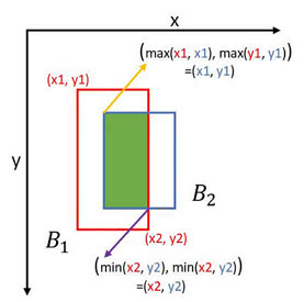
Then, to compute the area of the intersection, we multiply its height by its width.
To get the union of two boxes, we use the following equation:
union_area = box1_area + box2_area - intersection_area
Here is a function to compute IoU:
def iou(box1, box2):
    """Implement the intersection over union (IoU) between box1 and box2

    Arguments:
    box1 -- first box, list object with coordinates (x1, y1, x2, y2)
    box2 -- second box, list object with coordinates (x1, y1, x2, y2)
    """

    # Calculate the (y1, x1, y2, x2) coordinates of the intersection of box1 and box2. Calculate its Area.
    xi1 = max(box1[0], box2[0])
    yi1 = max(box1[1], box2[1])
    xi2 = min(box1[2], box2[2])
    yi2 = min(box1[3], box2[3])
    inter_area = (xi2 - xi1) * (yi2 - yi1)

    # Calculate the Union area by using Formula: Union(A,B) = A + B - Inter(A,B)
    box1_area = (box1[2] - box1[0]) * (box1[3] - box1[1])
    box2_area = (box2[2] - box2[0]) * (box2[3] - box2[1])
    union_area = box1_area + box2_area - inter_area

    # compute the IoU
    iou = inter_area / union_area

    return iou
The usefulness of Intersection over Union(
Non-max suppression is a common algorithm used for cleaning up when multiple boxes are predicted for the same object.
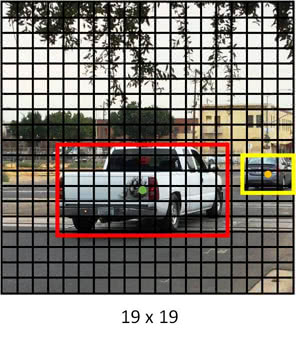
In our previous illustration, we use 3 x 3 bounding boxes. In reality, 19 x 19 bounding boxes are used to achieve a more accurate prediction. As a result, it's more likely to have multiple boxes predicted for the same object.
For the example below, the model outputs three predictions for the truck in the center. There are three bounding boxes, but we only need one. The thicker the predicted bounding box, the more confident the prediction is—that means a higher pc value.
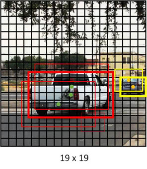
Our goal is to remove those "shadow" boxes surrounding the main predicted box.
That is what non-max suppression does in 3 steps:
And finally, the cleaned up prediction looks like this:
The YOLO model should now be ready to be trained with lots of images and lots of labeled outputs. Like the COCO dataset. But you won’t want to do
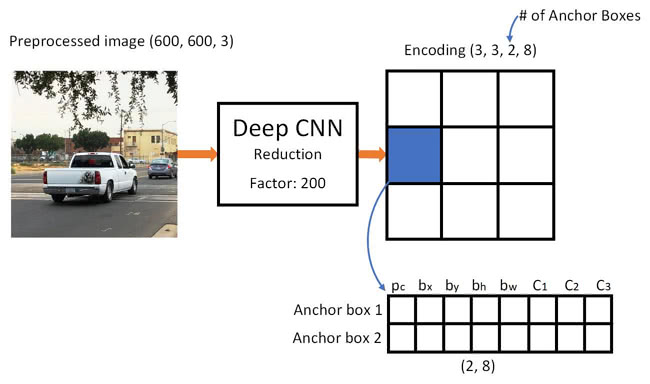
Before we get into the fun part, let's look at how the YOLO model makes predictions.
Given an image, the YOLO model will generate an output matrix of shape (3, 3, 2, 8). Which means each of the grid cells will have two predictions, even for those grid cells that don't have any object inside.
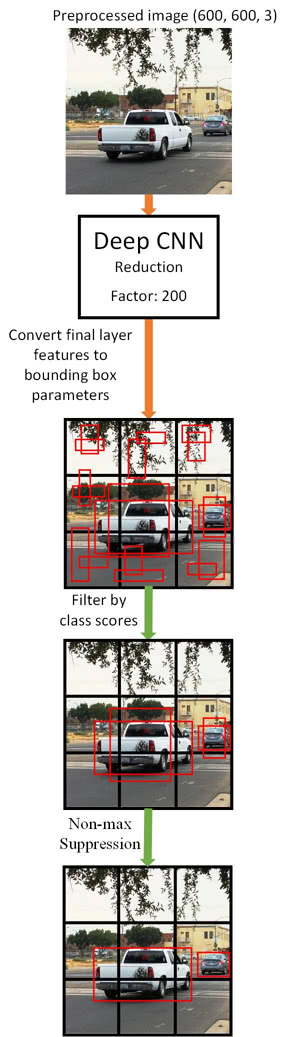
Before applying non-max Suppression to clean up the predictions, there is another step to reduce the final output boxes by filtering with a threshold by "class scores".
The class scores are computed by multiplying pc with the individual class output (C1, C2, C3).
So here is the graph illustrating the prediction process. Note that before "filter by class scores", each grid cell has 2 predicted bounding boxes.
With the previous concepts in mind, you’ll feel confident reading the YOLO model code.
The full source code is available in my GitHub repo. Let’s take a look at some parts worth mentioning.
Instead of implementing our own tf.image.non_max_suppression()
But wait, are we using a Keras model?
Not to worry. This time we’re using Keras backend API, which allows Keras modules you write to be compatible with TensorFlow API, so all TensorFlow operators are at our disposal.
from keras import backend as K
The TensorFlow+Keras implementation of non-max suppression can look like this. Note we are using a Keras variable and a TensorFlow operator here.
The input and output of the function are mostly input and output
def yolo_non_max_suppression(scores, boxes, classes, max_boxes = 10, iou_threshold = 0.5):
    """
    Applies Non-max suppression (NMS) to set of boxes

    Arguments:
    scores -- tensor of shape (None,), output of yolo_filter_boxes()
    boxes -- tensor of shape (None, 4), output of yolo_filter_boxes() that have been scaled to the image size (see later)
    classes -- tensor of shape (None,), output of yolo_filter_boxes()
    max_boxes -- integer, maximum number of predicted boxes you'd like
    iou_threshold -- real value, "intersection over union" threshold used for NMS filtering

    Returns:
    scores -- tensor of shape (, None), predicted score for each box
    boxes -- tensor of shape (4, None), predicted box coordinates
    classes -- tensor of shape (, None), predicted class for each box

    Note: The "None" dimension of the output tensors has obviously to be less than max_boxes. Note also that this
    function will transpose the shapes of scores, boxes, classes. This is made for convenience.
    """

    max_boxes_tensor = K.variable(max_boxes, dtype='int32')     # tensor to be used in tf.image.non_max_suppression()
    K.get_session().run(tf.variables_initializer([max_boxes_tensor])) # initialize variable max_boxes_tensor

    # Use tf.image.non_max_suppression() to get the list of indices corresponding to boxes you keep
    nms_indices = tf.image.non_max_suppression( boxes, scores, max_boxes_tensor, iou_threshold)

    # Use K.gather() to select only nms_indices from scores, boxes and classes
    scores = K.gather(scores, nms_indices)
    boxes = K.gather(boxes, nms_indices)
    classes = K.gather(classes, nms_indices)

    return scores, boxes, classes
And here is the code to construct the computation graph for prediction:
yolo_model = load_model("model_data/yolo.h5")
# Convert final layer features to bounding box parameters
yolo_outputs = yolo_head(yolo_model.output, anchors, len(class_names))
image_shape = K.placeholder(shape=(2, ))

# Retrieve outputs of the YOLO model
box_confidence, box_xy, box_wh, box_class_probs = yolo_outputs

# Convert boxes to be ready for filtering functions
boxes = yolo_boxes_to_corners(box_xy, box_wh)

# Perform Score-filtering with a threshold of score_threshold
scores, boxes, classes = yolo_filter_boxes(box_confidence, boxes, box_class_probs, threshold = score_threshold)

# Scales the predicted boxes in order to be drawable on the image.
boxes = scale_boxes(boxes, image_shape)

# Perform Non-max suppression with a threshold of iou_threshold
scores, boxes, classes = yolo_non_max_suppression(scores, boxes, classes, max_boxes = max_boxes, iou_threshold = iou_threshold)
We can then run the TensorFlow session to compute the output and finally draw predicted bounding boxes on the image.
# Preprocess your image
image, image_data = preprocess_image("images/" + image_file, model_image_size = (608, 608))

sess = K.get_session()

# Run the session with the correct tensors and choose the correct placeholders in the feed_dict.
out_scores, out_boxes, out_classes = sess.run([scores, boxes, classes], feed_dict={yolo_model.input: image_data,
                                                                                   input_image_shape: [image.size[1], image.size[0]],
                                                                                   K.learning_phase(): 0})

# Print predictions info
print('Found {} boxes for {}'.format(len(out_boxes), image_file))
# Generate colors for drawing bounding boxes.
colors = generate_colors(class_names)
# Draw bounding boxes on the image file
draw_boxes(image, out_scores, out_boxes, out_classes, class_names, colors)
# Save the predicted bounding box on the image
image.save(os.path.join("out", image_file), quality=90)
# Display the results in the notebook
output_image = scipy.misc.imread(os.path.join("out", image_file))
imshow(output_image)
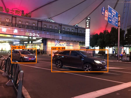
Here’s the output generated with a photo I took a while ago:
In this article, we walked through some key concepts that make the YOLO object localization algorithm work fast and accurately. Then we went through some highlights in the YOLO output pipeline implementation in Keras+TensorFlow.
Before wrapping up, I want to bring up 2 limitations of the YOLO algorithm.
YOLO: Real-Time Object Detection. This page contains a downloadable pre-trained YOLO model weights file. I will also include instruction on how to use it in my GitHub repo.
Allan Zelener - YAD2K: Yet Another Darknet 2 Keras. The Keras+TensorFlow implementation was inspired largely by this repo.
There are other competitive object localization algorithms like Faster-CNN and SSD. They share some key concepts, as explained in this post. Stay tuned for another article to compare these algorithms side by side.
Share on Twitter Share on Facebook
Comments